
SOM (Self Organizing Map)
1. Basic concept of the Self Organizing Map(SOM)
 A self-organizing map(SOM) is a type of artificial neural network(ANN) that uses unsupervised learning to produce a low-dimensional neural outputs.
But SOMs are little bit different from other ANNs in that they use a neighborhood function to preserve the topological properties of the input space. It consists of components called nodes or neurons like other ANNs. Each node is a weight vector of the same dimension as the input data vectors and a position in the map space.
The procedure of placing a vector from data set onto the map is to find the node with the closest weight vector, called winning neuron from the data space. Once the closest node is located than we can get new weight vector set. Finally we obtain updated output weight vectors that are trained and categorized. Once we have an unseen input than we can categorize or recognize the character by using weight vectors.
2. Summary of the SOM algorithm
Step 1. Initialize parameters such as weight vectors  ,
,
,


Step 2. Check stopping condition
Step 3. For each training vector x, perform steps 4 through 7.
Step 4. Compute the best match of a weight vector with the input
Step 5. For all units in the specified neighborhood  , update
, updatethe weight vectors according to
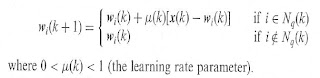
Step 6. Adjust the learning rate parameter.
Step 7. Appropriately reduce the topological neighborhood  (k)
(k)
(k)Step 8. Set k <- k+1; then go to step 2.
3. Simulation setting
We can simulate the SOM algorithm by using given various data set of characters.

We have 2500 image data set that is sufficient to obtain reasonable weight vectors. Appropriately I let learning rate parameter to 0.0005, initially. It becomes 1 finally.
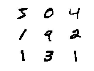
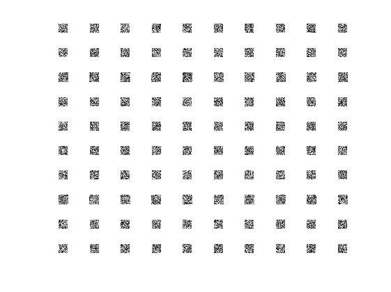
Input images consist of 784 nodes and actually it is a 28*28 matrix like below.
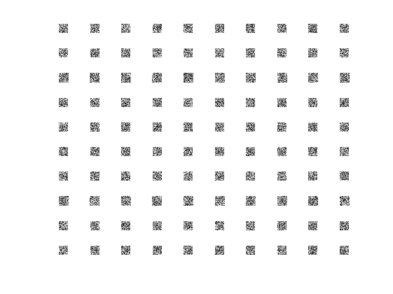
We can make arbitrary random initial weight vectors.

They will be updated and become meaningful image set.
5 Find winner neurons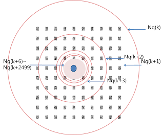
4. Source Code
To verify the algorithm I composed some matlab codes.
Source codes
% main.m %% initialize %% sample_No = 2500; % # of samples eta_i = 0.0005; % initial learning rate eta = eta_i; % learning rate w = rand(28, 28, 100); % initial weight vector k = 0; %% update the synaptic weight vectors for k = 1:2500 % culculate q(x) ------------------ x = reshape(data(k,:), 28, 28); [index] = evaluate_q(x,w); %---------------------------------- [x_point, y_point] = find_grid(index); % find x,y points of winning neuron for x_index = 1:10 for y_index = 1:10 % decide within Nq sub = [x_point-x_index y_point-y_index]; n = norm(sub,2); if(n<150000*exp(-1-4*(k/sample_No*5))) % update weight vectors if within Nq grid = (x_index-1)*10+y_index; w(:,:,grid) = w(:,:,grid) + eta*(x-w(:,:,grid)); end end end % update learning rate eta = eta_i + 0.0004*k; end |
function [index] = evaluate_q(x,w) min = 1000; for i = 1:100 wj = w(:,:,i); n = norm(x-wj,2); if(min>n) min = n; index = i; end end |
function [x, y] = find_grid(index) x = floor(index/10); y = index - x*10; |
5 Find winner neurons
To find best match vector I used 2-norm function such as n = norm(x-wj,2); It worked well and also I could get the index 'i' of Weight vector.
6 Neighborhood function
I used a circle model rather than a hexagon model. Because It is simple and It has good performance as well. At first neighborhood function covers all of weight vectors since it is big enough wherever it is located.
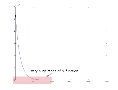
Neighborhood function become smaller exponentially that is it is updated exponentially. I used exponential function to update the Neighborhood function.
150000*exp(-1-4*(k/sample_No*5))
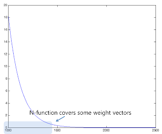
I just appropriately reduced the topological neighborhood Nq(k). First 40% of k neighborhood function cover all of the weight vectors. The graph is below
In 1000< k <2500, N-function covers some weight vectors
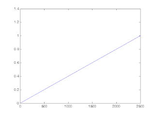
7 Learning rate
Leaning rate increase from 0.005 to 1 linearly. At first the range of neighborhood function is so huge. So learning rate need to be small enough. Finally leaning rate becomes 1 as neighborhood function range becomes small.
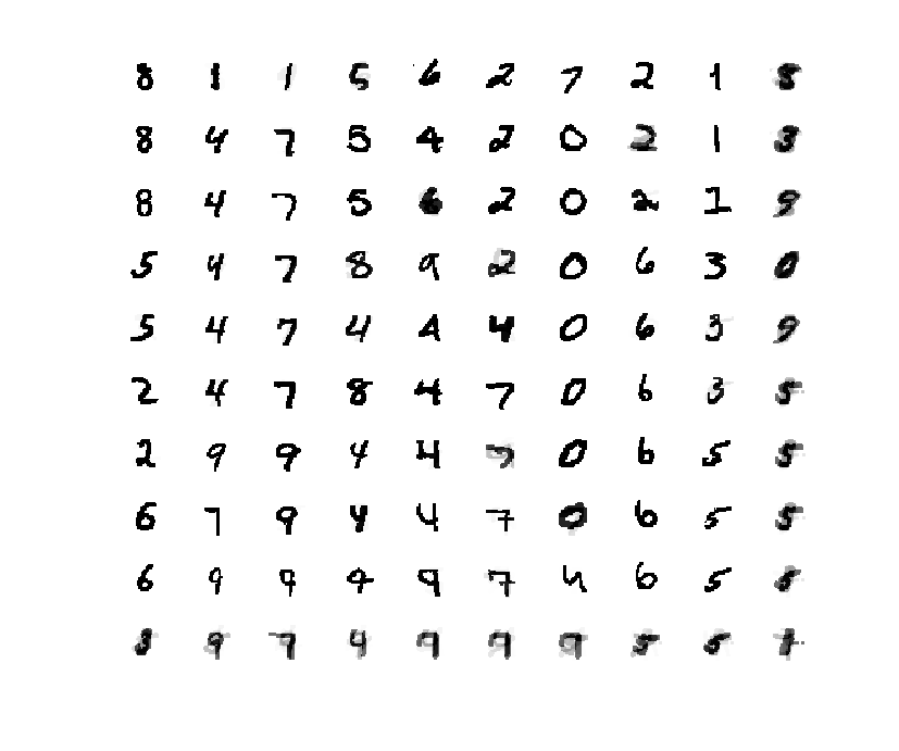
8 Result
  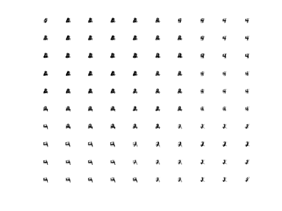 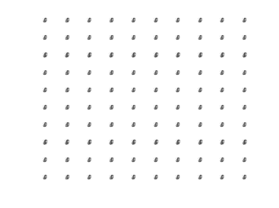 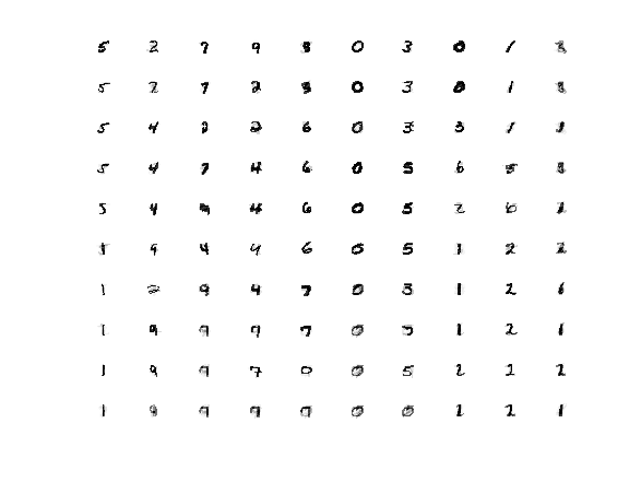 |
After 2500 iterations, the weight vectors are formed like legible characters.
If there are unseen data set, we can classify them by using weight vectors
댓글남기기